Assess
The purpose of this chapter is to assess whether integrating the multiSolve library in your project is worth your while. The multiSolve library is most effective for batches of solving mathematical programs, whereby
there are several solves that can be executed simultaneously,
a solver and license are used that permit asynchronous solving,
increasing the number of threads per solve does not improve significantly the time needed for that solve, and
the solving time by the solver of an instance dominates the time needed by the AIMMS Execution Engine for that instance.
Admittedly, this is a significant number of requirements. Lets examine them in some detail.
Simultaneous solving permitted.
Two GMP’s, say ep_gmpA and ep_gmpB can be solved simultaneously when the solution of ep_gmpA
does not influence the generation of ep_gmpB and visa versa.
In steps an example is given when some GMP’s depend on each other, and some are independent. In that case, the multiSolve library can still be of use.
Solver and license permit asynchronous solving
The multiSolve library assumes the CPLEX solver with a license for asynchronous (parallel) solving. A license for asynchronous solving is an extended license. Please contact info@aimms.com for further details.
Increasing number of threads does not speedup a single solve
Some solvers make effective use of multiple logical processors to speedup the solving. A typical example is a MIP whereby most of the time is spent in the branch and cut phase.
To avoid thread starvation, the number of threads allotted to a solve times the number of parallel solves should not exceed the number of logical processors.
To determine whether the mathematical programs solved by your application are benefiting from multi-threaded solving, you can test by setting the CPLEX option global_thread_limit to 1.
When the solve time significantly increases by setting this limitation to the solver, your application is automatically benefiting from the availability of multiple logical processors. When this is the case, there is only value to the multiSolve library when the number of logical processors available meets the speedup of multi-threaded solving by the factor of the number of solves you want to be executed in parallel.
The solve time dominates the total time
The multiSolve time reduces the wait time on actual solving. Therefore, if the time spent on actual solving is a small fraction of the total time, the integration may not be worthwhile. However, lets look at some detail here:
Understanding the sub components of AIMMS relevant to multiSolve
Within a single AIMMS process, there is:
at most one AIMMS Execution Engine active, and
there are 0, 1, or more solvers active.
The following tasks relevant to using the multiSolve library occur within the AIMMS Execution Engine.
Obtaining the data for every instance to be solved.
Generating or modifying a GMP corresponding to the data instance at hand.
Obtaining the solution of a solved GMP, and storing that in the data structures of the application.
To predict the speed up of using multiSolve, it is important to know and compare the
time needed to execute the above three tasks, dubbed EngineTime below, and
time needed to solve a GMP, dubbed SolveTime below.
Knowing the EngineTime and the SolveTime
In this section, two situations are considered:
Your application uses a solve statement to solve mathematical programs.
Your application uses GMP technology to generate and modify GMP’s.
Determining the Enginetime and the SolveTime starting with a solve statement
A solve statement combines the time to generate a mathematical program and the time needed to actually solve that mathematical program. The time needed to generate is part of the EngineTime. The time needed to actually solve, is the SolveTime.
Each of the following techniques can be used to separate generation time from the solver time:
Make the solve statement, two statements using the GMP technology. Then do a run using the AIMMS Profiler. In more detail:
First declare the element parameter
ep_gmp, with rangeAllGeneratedMathematicalPrograms.Then replace a solve statement like:
solve myMathProg ;
with
ep_gmp := gmp::instance::generate( myMathProg );
gmp::instance::solve( ep_gmp );
A run with an AIMMS Profiler on, may then give the following:
Check the suffices gentime and solutionTime of a Mathematical Program
Check the solver log file for the time needed by the solver, and the time needed to generate is the time for the solve statement minus the time reported by the solver.
Determining the Enginetime and the SolveTime when using GMP technology.
When your application is using GMP functionality to generate and/or modify Generated Mathematical Programs:
Provide Generate mode
Provide Modify mode
Comparing the EngineTime and the SolveTime
Consider the following three situations comparing EngineTime and SolveTime:
EngineTime >> SolveTime (EngineTime is relatively significantly more than the SolveTime). In this situation the improvement to the wall clock time will be relatively small.
EngineTime ~ SolveTime (EngineTime is comparable to SolveTime). In this situation, effectively there is one solver running in parallel to the AIMMS Execution Engine; as soon as the AIMMS Execution Engine is able to handle a next instance, the solver will be ready to handle the solving of a new instance. The speed up will likely be almost a factor of 2.
To illustrate consider the following graph on CPU load:
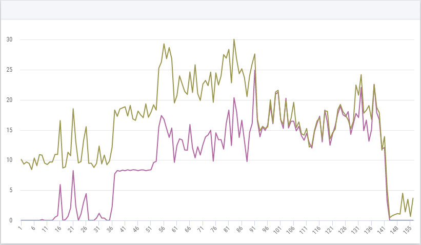
The olive colored top line is the CPU load of all processes during the session, the purple colored bottom is the CPU load by the entire AIMMS process (so including the solves active).
To create this graph, the Blend example was solved in
generateprovide mode. In this mode, it takes significant time to generate a new GMP, and the EngineTime time becomes comparable to SolveTime. During that AIMMS Session, the Windows Utility PerfMon was used to measure the CPU load.Remarks on the graph:
At second 35 the first GMP is generated and solved for another ten seconds or so. This is actually outside the use of multiSolve.
At second 51, the multi solve becomes active, first generating and then combining generation and solving.
EngineTime << SolveTime (EngineTime is significantly less than the SolveTime). In this situation, there can be up to eight solver session active while the AIMMS Execution Engine is actually waiting of one of them to finish.
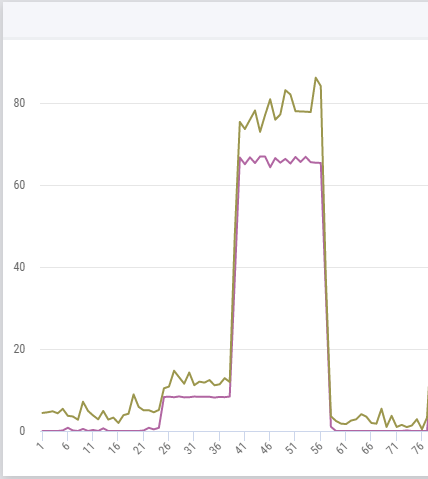
The olive colored top line is the CPU load of all processes during the session, the purple colored bottom is the CPU load by the entire AIMMS process (so including the solves active).
To create this graph, the Blend example was solved in
modifyprovide mode. In this mode, it hardly takes time for AIMMS Execution Engine to provide a new GMP based on the new objective coefficients, enabling it to start up several solves before the first solve finishes.Remarks on the graph:
At second 25 the first GMP is generated and solved for another ten seconds or so. This is actually outside the use of multiSolve.
At second 38, the multi solve becomes active, first generating and then combining generation and solving. Clearly, the CPU load is much higher than in the previous graph, as there are now several solves active at the same time.
In short, by switching the provide mode to 'generate', the integration of the multiSolve becomes much more valuable.