Quick Start: My First WebUI App
This section illustrates how to create quickly a first Web-based User Interface (WebUI) for a simple Transport Network (TransNet) application using a set of locations divided in two (disjoint) subsets of factories and distribution centers. Each factory has an amount of supply of a product and each distribution center has some demand for that product. Decisions have to be made on how much to transport from a factory to a distribution center in order to satisfy demand, while not exceeding the available supply. Unit transport costs are associated with any pair of factory and distribution center and the transport decisions aim to minimize the total transport cost for the entire network.
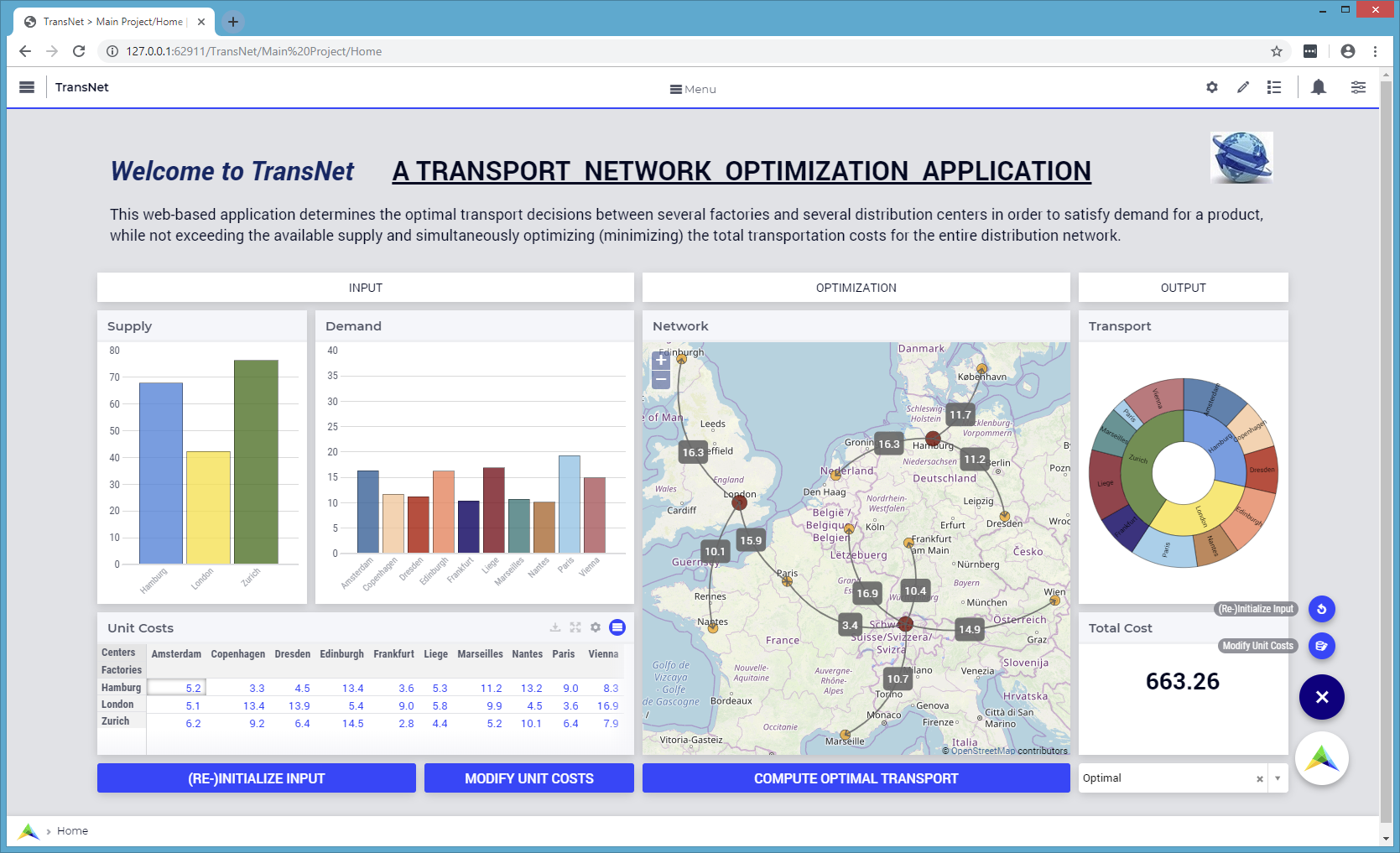
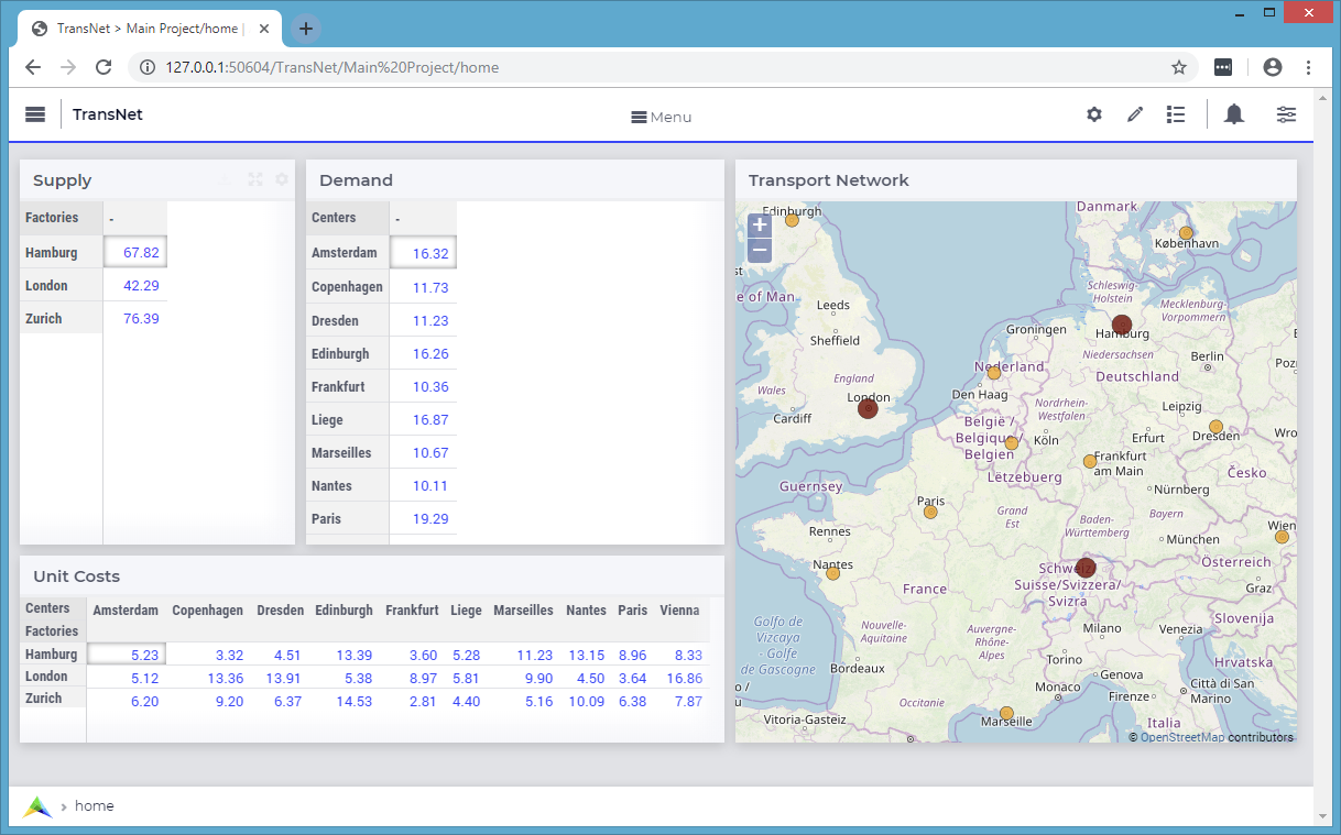
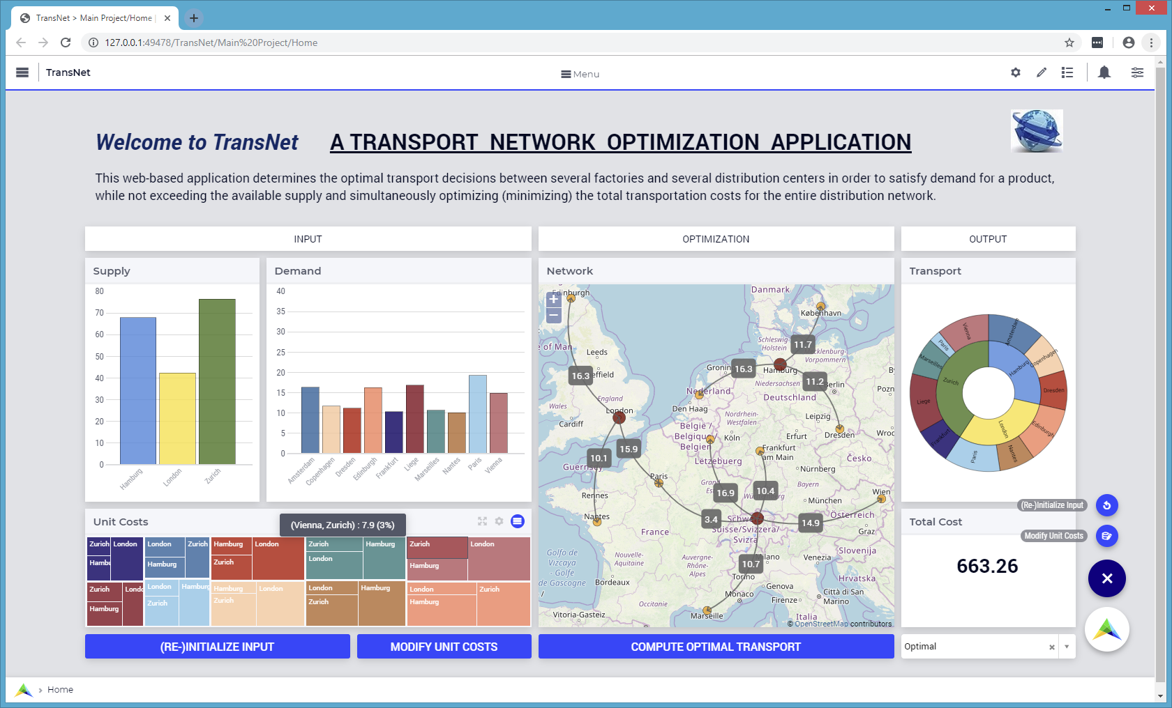
A first WebUI for such an AIMMS optimization application may look like in the following picture:
In order to build such a WebUI, one needs to add and configure step-by-step a number of widgets on the Home application page opened in a browser tab. Most widgets reference data of identifiers or run procedures present in the AIMMS model.
The underlying optimization model
In the sequel, some code snippets from the underlying AIMMS model show identifiers from the model declarations. The declarations for the network locations look as follows:
DeclarationSection Network_Locations {
    Set Locations {
        Index: l;
    }
    Parameter Latitude {
        IndexDomain: l;
    }
    Parameter Longitude {
        IndexDomain: l;
    }
    Parameter IsFactory {
        IndexDomain: l;
        Range: binary;
    }
    Parameter IsCenter {
        IndexDomain: l;
        Range: binary;
        Definition: 1 - IsFactory(l);
    }
}
Subsequently, the following model declarations concern the input data for the model:
DeclarationSection Input_Data {
    Set Factories {
        SubsetOf: Locations;
        Index: f;
        Definition: {
            { l | IsFactory(l) }
        }
    }
    Set Centers {
        SubsetOf: Locations;
        Index: c;
        Definition: {
            { l | IsCenter(l) }
        }
    }
    Parameter Supply {
        IndexDomain: f;
    }
    Parameter Demand {
        IndexDomain: c;
    }
    Parameter UnitCost {
        IndexDomain: (f,c);
    }
}
In the use case at hand, there are 3 factories (Hamburg, London, and Zurich) and 10 distribution centers (Amsterdam, Copenhagen, Dresden, Edinburgh, Frankfurt, Liege, Marseille, Nantes, Paris, and Vienna). The input data may be initialized upon the application start-up by using some simple procedures. The Latitude and Longitude parameters, as well as the IsFactory binary indicator parameter may be initialized in a procedure by using e.g., a composite table (or, alternatively, by reading in their values from an external source):
Procedure Initialize_Network {
    Body: {
        COMPOSITE TABLE:
        l                Longitude      Latitude     IsFactory
        !-----------------------------------------------------
        Amsterdam          4.88           52.38
        Copenhagen        12.54           55.66
        Dresden           13.74           51.05
        Edinburgh         -3.19           55.95
        Frankfurt          8.71           50.17
        Hamburg            9.98           53.54           1
        Liege              5.58           50.63
        London            -0.16           51.50           1
        Marseille          5.38           43.29
        Nantes            -1.55           47.22
        Paris              2.34           48.86
        Vienna            16.37           48.20
        Zurich             8.54           47.37           1     ;
    }
}
The Supply and Demand parameters may be initialized e.g., by using some random draws from uniform distributions, while the parameter UnitCost may be initialized e.g., based on the (straight line) distance between two locations (see further below).
Creating an empty WebUI
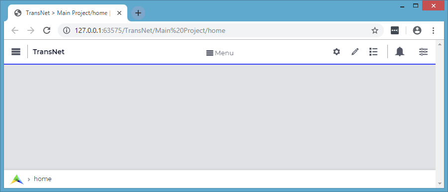
One may start by opening the Home page of the WebUI application in the browser (see Create a WebUI section for details):
Adding the widgets for input data
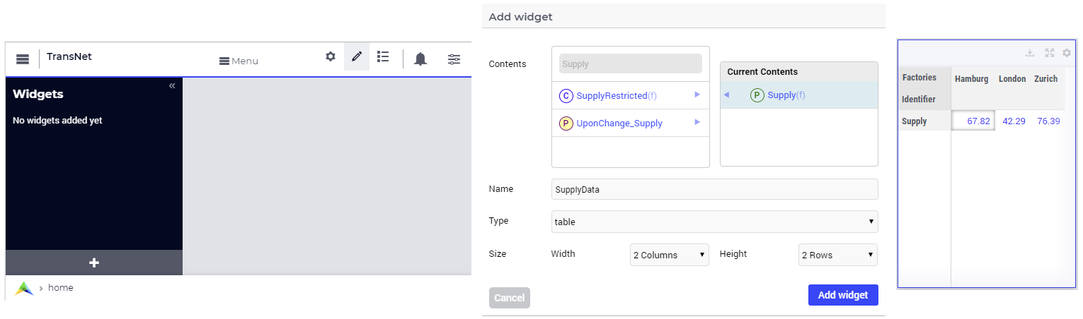
On this page one can add widgets for rendering the data of the input parameters Supply and Demand. For example, one can add a table widget named “SupplyData” with sizes of 2 columns and 2 rows, rendering the data of the parameter Supply. In the Widget Manager, pressing the “+” sign at the bottom opens the “Add widget” pop-up window, where the fields can be filled in as shown below, resulting in a widget like here on the right hand side:
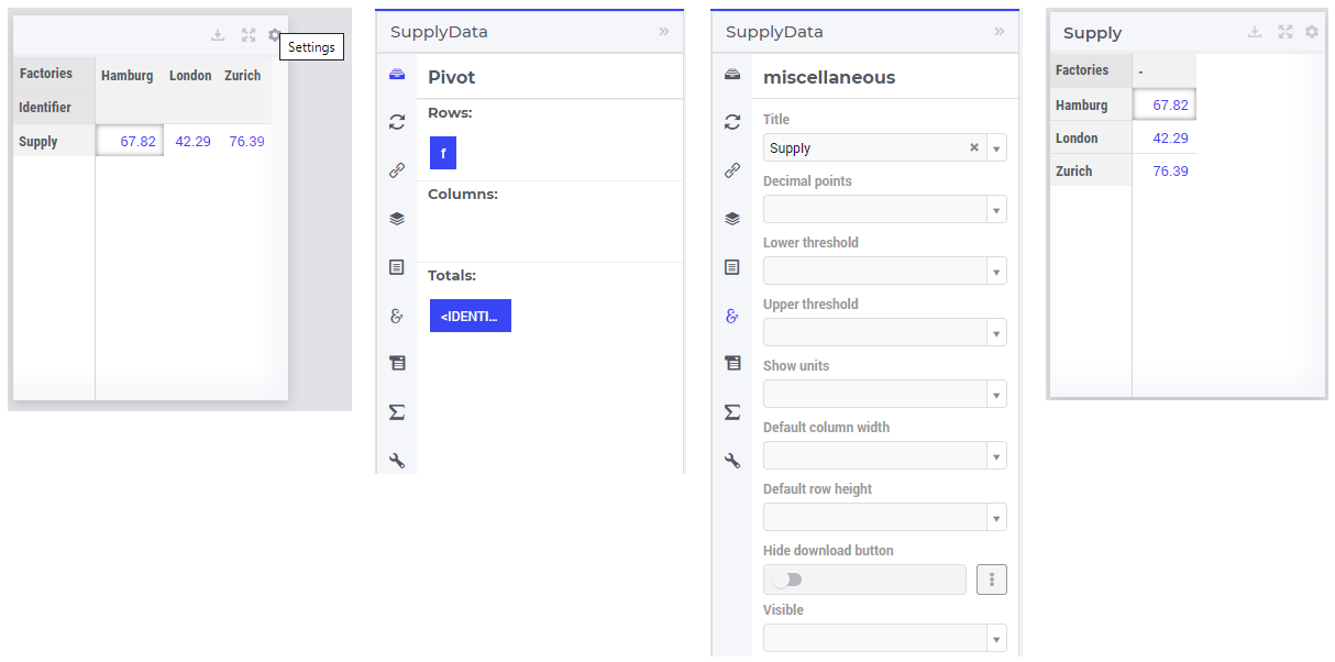
The SupplyData widget can be further configured in its Settings window, for example by swapping indexes in the Pivot section or by typing the title Supply in the Miscellaneous section, as illustrated below. After these steps, the SupplyData table should look like in the last picture on the right hand side below:
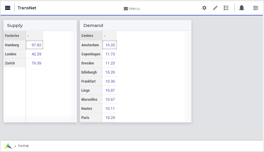
In a very similar manner, one can undertake steps as above for adding and configuring a second table widget named “DemandData” with sizes of 3 columns and 2 rows (title Demand), rendering the data of the parameter Demand. The two added table widgets should now look like in the following picture:
Next one can add a map widget with 4 columns and 3 rows (title Transport Network) in order to show the locations of the network. The map widget can be added by using the same “Add widget” window as discussed before. Then in the Settings window of the map widget the Node Sets and the Miscellaneous sections can be filled in as shown below, resulting in a map widget as here on the right:
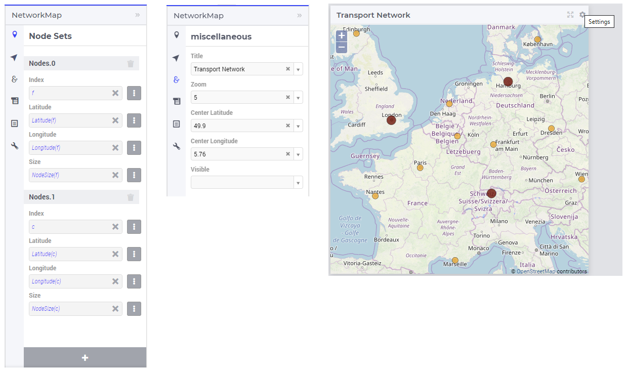
As shown in the snapshots above, two types of nodes have been added explicitly to the network in the map widget: one type for the factories f and one other type for the distribution centers c. Please note that for specifying the Latitude, the Longitude and the NodeSize corresponding to each of the indexes f and c, the slicing functionality (as described in the Slicing section) can be used.
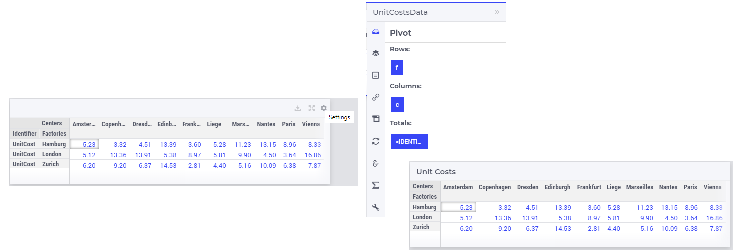
Another table widget with 5 columns and 1 row (title Unit Costs) may be added for showing the unit transport costs between a factory and a distribution center. The widget tile may be added in the same way as above, while the splitting of indexes of this parameter between the row area and the column area may be configured in the Pivot section of the Settings window as illustrated below:
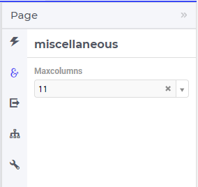
In the Miscellaneous section of Page Setting window, one can set a maximum number of 11 columns for the page as shown here:
After performing all the steps so far, the WebUI should look like in the following picture:
Including widgets for optimization and output data
The mathematical optimization declarations in the AIMMS model look as follows:
DeclarationSection Optimization_Model {
    Variable Transport {
        IndexDomain: (f,c);
        Range: nonnegative;
    }
    Variable TransportCost {
        Range: free;
        Definition: sum[ (f,c) , UnitCost(f,c) * Transport(f,c) ];
    }
    Constraint SupplyRestricted {
        IndexDomain: f;
        Definition: sum[ c, Transport(f,c) ] <= Supply(f);
    }
    Constraint DemandRequired {
        IndexDomain: c;
        Definition: sum[ f, Transport(f,c) ] >= Demand(c);
    }
    MathematicalProgram TransportModel {
        Objective: TransportCost;
        Direction: minimize;
        Constraints: AllConstraints;
        Variables: AllVariables;
        Type: Automatic;
    }
}
Some additional declarations for the model output can be added as follows:
DeclarationSection Output_Data {
    Parameter IsTheModelSolved {
        Range: binary;
    }
    Set LP_ModelStatuses {
        SubsetOf: AllSolutionStates;
        Definition: data{ 'Optimal', 'Infeasible', 'Unbounded', 'SolverNotCalled' };
    }
    ElementParameter TransportModelStatus {
        Range: LP_ModelStatuses;
        Definition: {
            if IsTheModelSolved
               then TransportModel.ProgramStatus
               else 'SolverNotCalled'
            endif;
        }
    }
}
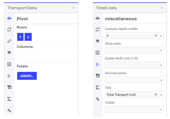
For output data one may add to the Home page in the WebUI a table widget with 2 columns and 2 rows (title Transport) showing the data of the Transport variable and a scalar widget with 2 columns and 1 row (tile Total Transport Cost) rendering the data of the variable TransportCost. The Settings of these two widgets may be configured as shown in the following two pictures, respectively:
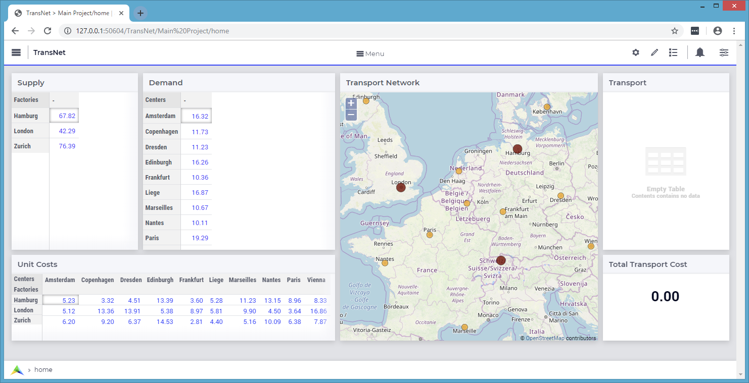
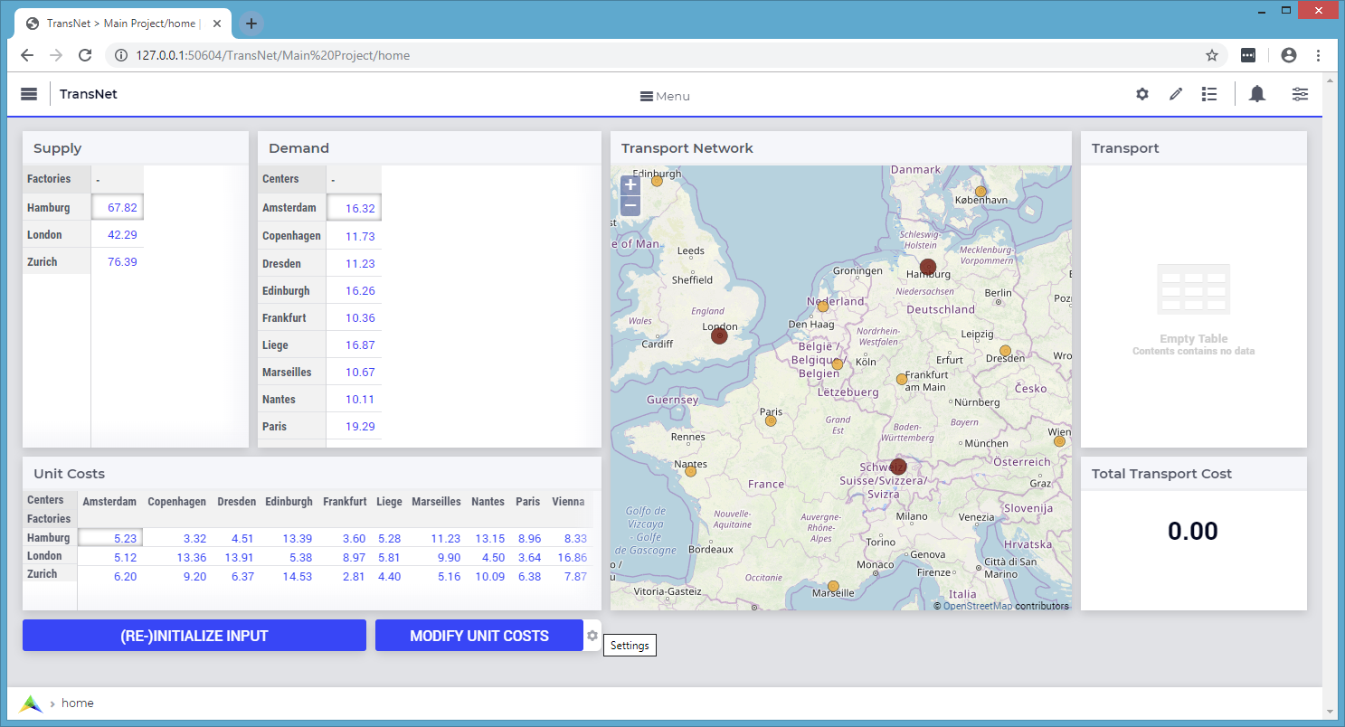
The last two widgets have no data to be shown before the model is solved, so, after performing also the last steps, the WebUI should look as follows:
Adding buttons
The procedures which initializes the input state before solving the model may be declared for example like here:
Procedure Initialize_Input {
    Body: {
        option seed = 1234;

        Supply(f) := Round( Uniform(40,80), 2 );
        Demand(c) := Round( Uniform(10,20), 2 );

        Initialize_UnitCosts;

        Empty_Variables;
    }
}

Procedure Initialize_UnitCosts {
    Body: {
                UnitCost(f,c) := Round( Sqrt(Sqr(Latitude(f)-Latitude(c)) + Sqr(Longitude(f)-Longitude(c))), 2 );
    }
}
where the procedure Empty_Variables called above simply empties the output state:
Procedure Empty_Variables {
    Body: {

        empty Transport, TransportCost, IsTheModelSolved;
    }
}
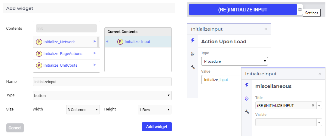
On the WebUI page one can now add a button widget with 3 columns and 1 row (tile (RE-)INITIALIZE INPUT) and configure it in the Action section of its Settings window in order to run upon click the procedure Initialize_Input as illustrated below:
In order to experiment using other unit transport costs than the initial ones, a procedure as the following may be used:
Procedure Modify_UnitCosts {
    Body: {

        Initialize_UnitCosts;

        option seed = 5678;

        UnitCost(f,c) *= Uniform(0.3,2.5);

        Empty_Variables;
    }
}
Similarly as before, one can add another button widget with 2 columns and 1 row (title MODIFY UNIT COSTS) running upon click the last procedure mentioned above. After performing all the steps so far, the WebUI page should look like shown below:
Solving the optimization model
Now it is time to actually solve the optimization model and show the resulting output data in the WebUI. In developer model, solving the model normally requires a simple procedure as the following:
Procedure Solve_Model {
    Body: {

        solve TransportModel;

        IsTheModelSolved := 1;

        !If the problem was not solved to optimality, make sure that the decision variables
        !are emptied, because they do not correspond to an actual solution.

        if ( TransportModelStatus <> 'Optimal' ) then
            empty Transport, TransportCost  ;
        endif ;
    }
}
However, in case the application is run on AIMMS PRO, the WebUI client needs to delegate the optimization procedure to the solver session running on the PRO server using a procedure as the following:
Procedure Solve_Delegate {
    Body: {

        if pro::DelegateToServer( waitForCompletion : 1, completionCallback : 'pro::session::LoadResultsCallback' )
           then return 1;
        endif ;

        SolveModel;
    }
}
So, the overall solving procedure which addresses all situations (developer mode and deployment PRO mode) can be declared like shown below:
Procedure Solve_Procedure {
    Body: {

        if ProjectDeveloperMode then

               Solve_Model;

        elseif pro::GetPROEndPoint() then

                if pro::IsRunningAtServer then

                   Solve_Model;

                else

                   Solve_Delegate;

                endif;
        endif ;
    }
}
After making sure that the above declarations are present in the AIMMS model, one can add to the WebUI a new button widget with 4 columns and 1 row (title COMPUTE OPTIMAL TRANSPORT) running upon click the last procedure mention above, which actually solves the transport optimization model.
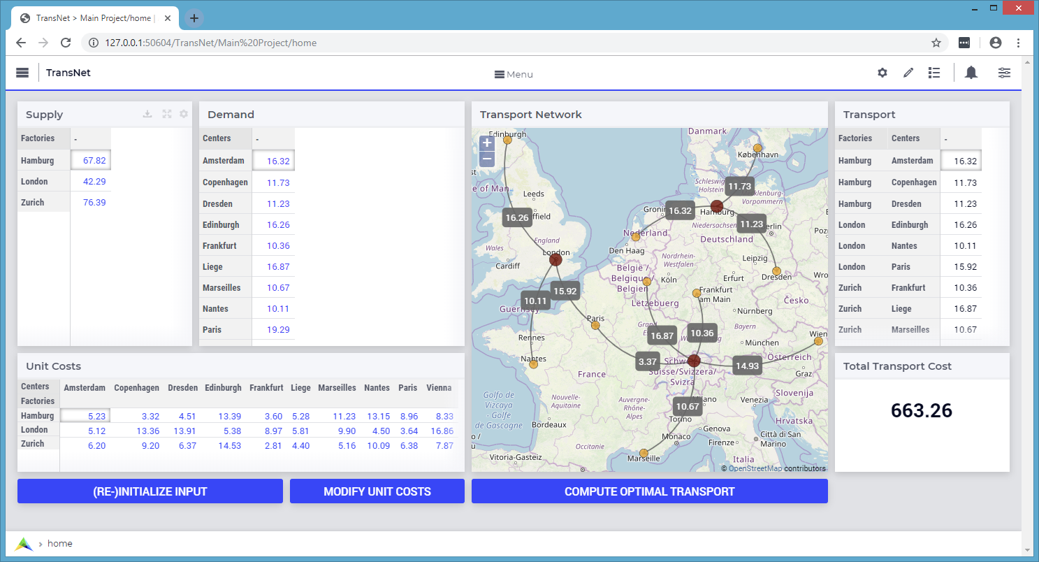
So, after pushing this button the output data is filled in for the Transport table and the Total Transport Costs scalar. However, the Transport amounts are not yet shown in the map widget. In order to achieve this, one needs to open the Settings window of the map widget and add the arcs in the Map Contents section of as follows:
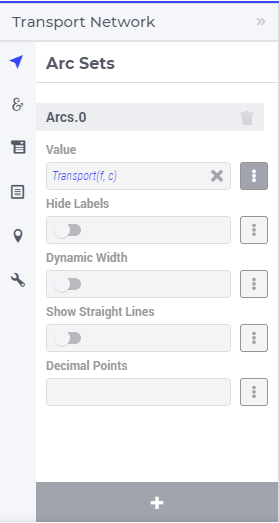
So, after performing all the steps so far the WebUI should look as shown here:
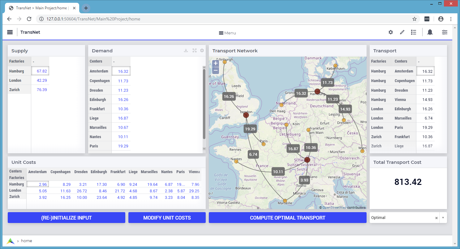
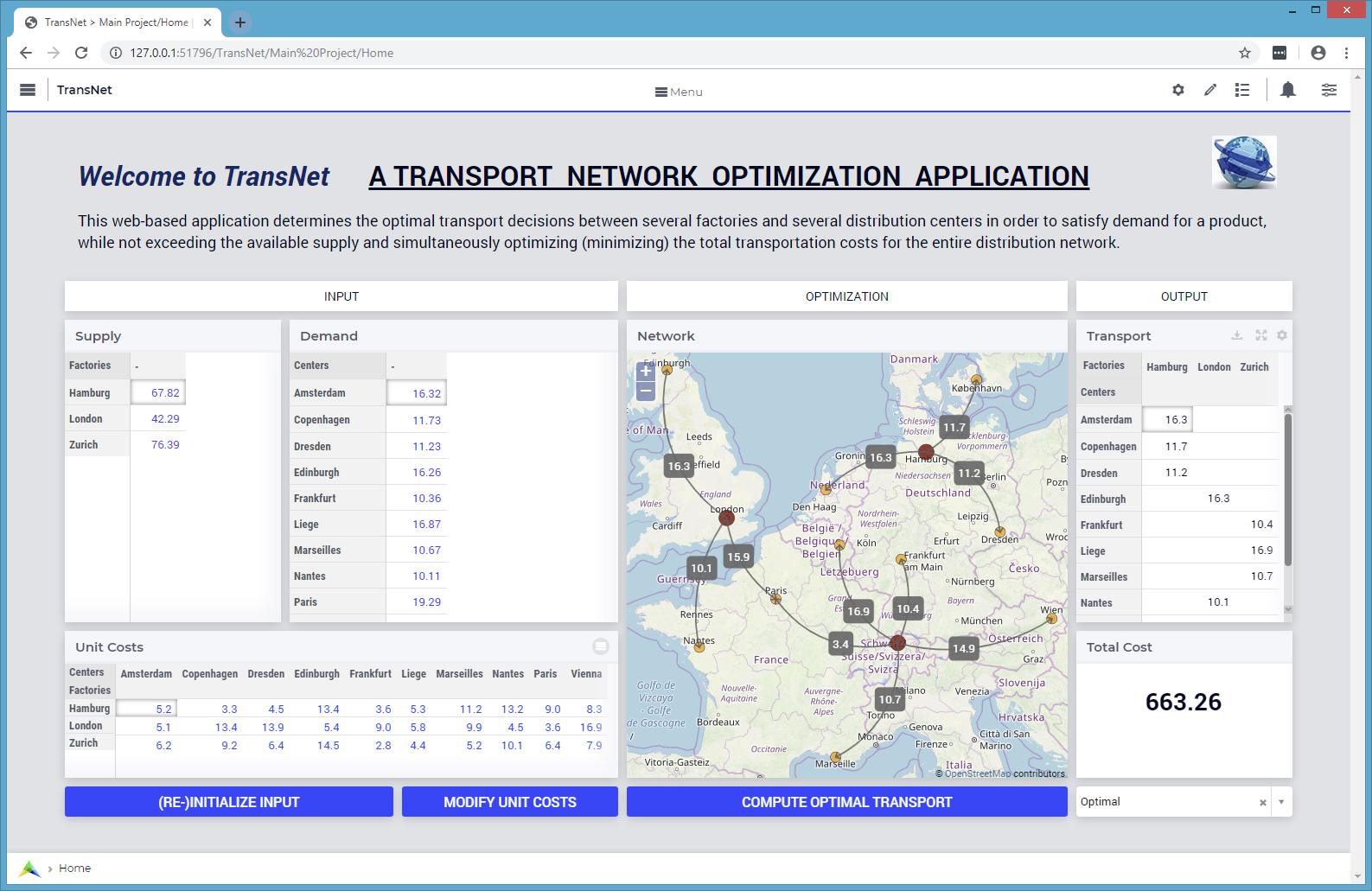
One may add to the WebUI a selectionbox widget with 2 columns and 1 row showing the value of the element parameter TransportModelStatus. After pushing the “MODIFY UNIT COSTS” button and then solving the model again by using the “COMPUTE OPTIMAL TRANSPORT” button, the WebUI overview should now show the new solution (with visible model status Optimal ) as in the following picture:
Providing more structure to the WebUI
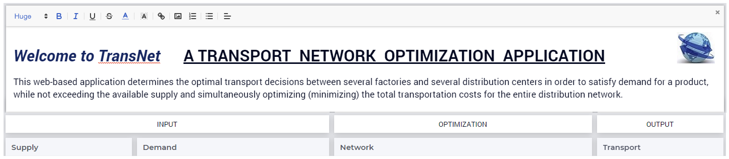
In order to indicate more clearly the input, the optimization, and the output parts in the WebUI, one may add 3 label widgets called InputLabel (contents INPUT), OptimizationLabel (contents OPTIMIZATION), and OutputLabel (contents OUTPUT), in this order. All labels can have 1 row, while the columns sizes may be 5 columns, 4 columns, and 2 columns, respectively. The label widgets may be moved up (by drag-and-drop) as the first 3 widgets in the Widgets Manager, in the same order, while the rest of the widgets may follow up by keeping their relative order in which they have been added. Furthermore, a new text widget with 11 columns and 1 row may also be added as the very first widget in the Widget Manager in order to show a title / introduction section for the entire application (like the one shown in the first overview picture in the very beginning of this documentation section). Formatting the contents of such a text widget is self-explanatory in its Edit window by using the options on the top:
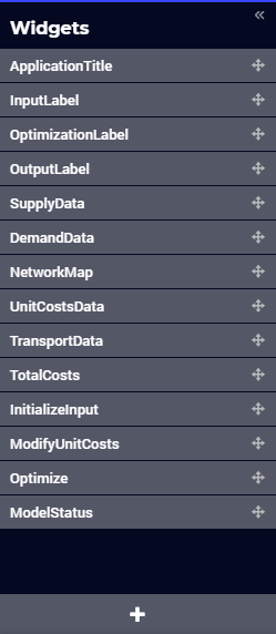
The final Widget Manager showing all widgets and their relative order looks like shown here:
After pushing again the input initialization button and the optimization button, one should retrieve the initial solution and the WebUI should look as follows:
Performing What-If analysis
One can perform a “What-If” type of analysis by changing values for Supply, Demand, or UnitCosts, and subsequently re-solving the model. When input data changes, it may be handy to empty right away the output data resulted from the previous runs. This can be achieved by declaring procedures with names starting with “UponChange_” followed by the name of the identifier which incurs a change, similar to the ones below:
Procedure UponChange_Supply {
    Body: {
                Empty_Variables;
    }
}

Procedure UponChange_Demand {
    Body: {
                Empty_Variables;
    }
}

Procedure UponChange_UnitCost {
    Body: {
                Empty_Variables;
    }
}
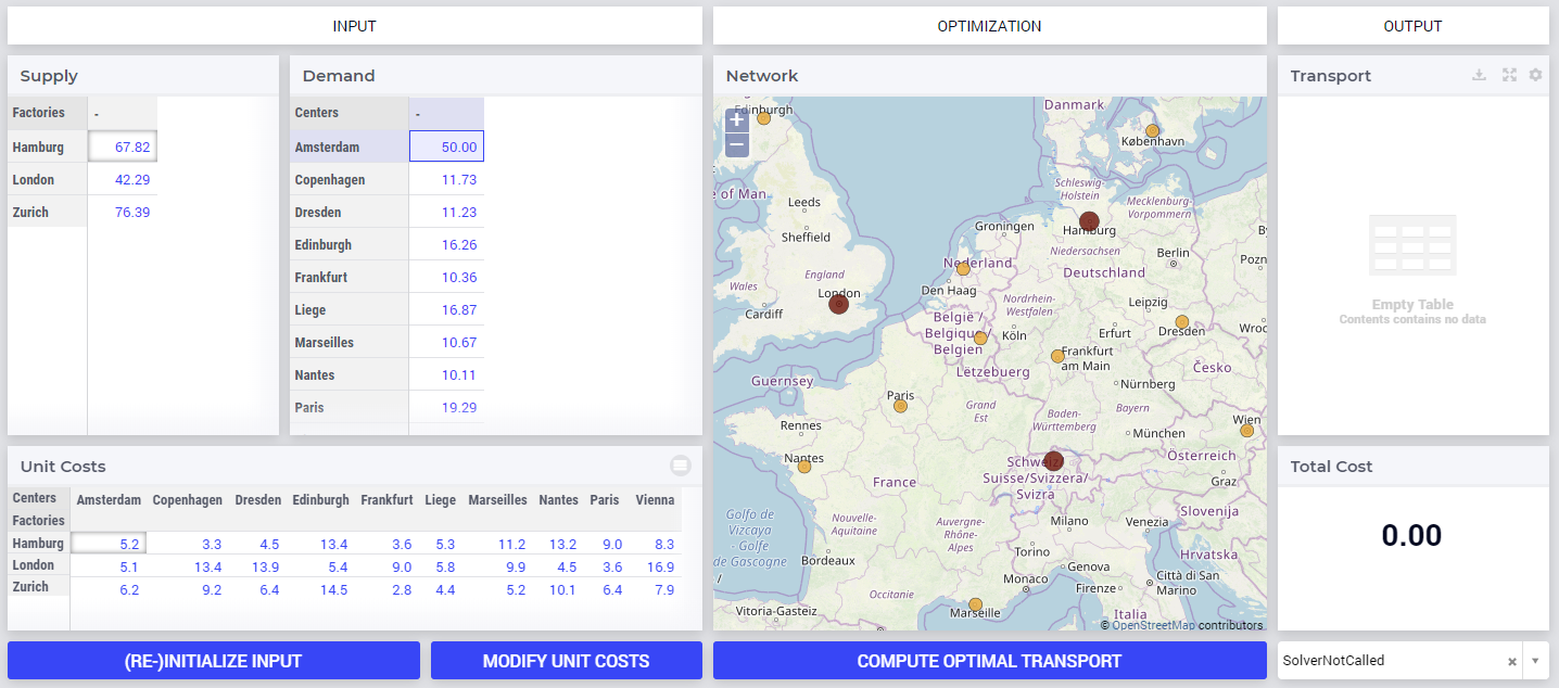
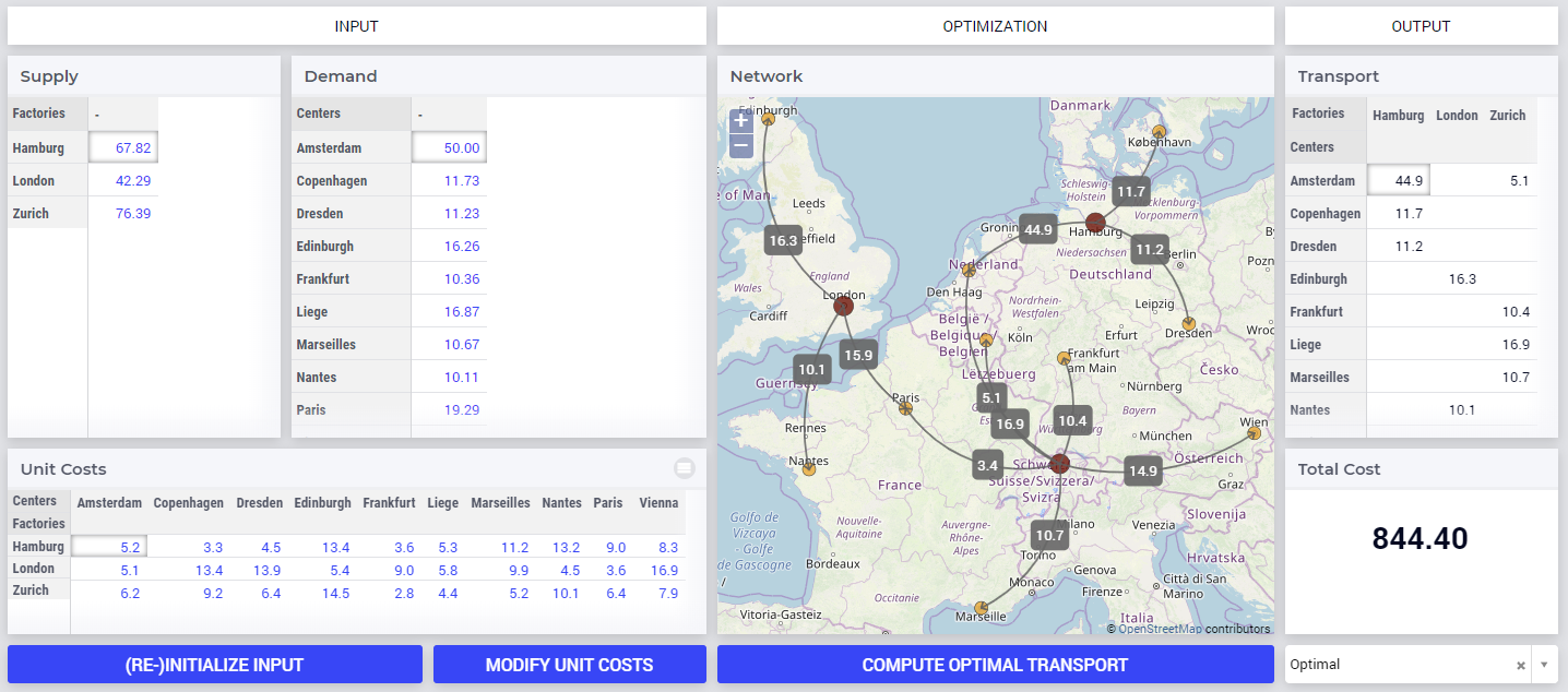
One may change for example, the Demand value in Amsterdam to 50 and this action will also empty the widgets for output data and show in the model status that the solver has not been called yet:
After pushing again the “COMPUTE OPTIMAL TRANSPORT” button, the new solution is shown and the model status becomes Optimal again:
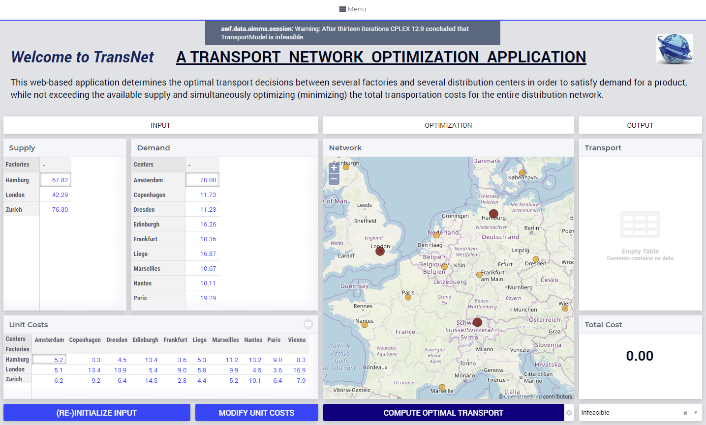
One may try and repeat the experiment for the scenario in which Demand value in Amsterdam would increase, for example, to 70. In this case the model becomes infeasible, because the total demand exceeds the total available supply. So, the output data stays empty and the model status is set to Infeasible:
Of course, one may experiment with several scenarios by altering (also simultaneously) several values in Supply, Demand, and UnitCosts, re-solving the model and observing the impact of the new input to the model status and the solution, in case the model is feasible.
Saving and comparing cases
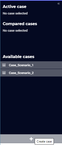
Any such scenario (as discussed above) may be saved as a data case using the Data Manager. For example, one may re-initialize input, then optimize, and then save the corresponding scenario as Case_Scenario_1. Similarly, one may modify input, then optimize, and then save the resulting scenario as Case_Scenario_2 in the Data Manager:
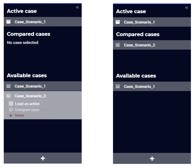
Any saved case may be loaded as the active case using the Data Manager:
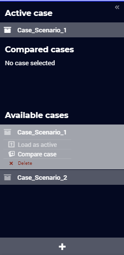
Once a case has been loaded as active, another saved case may be compared to the currently active case:
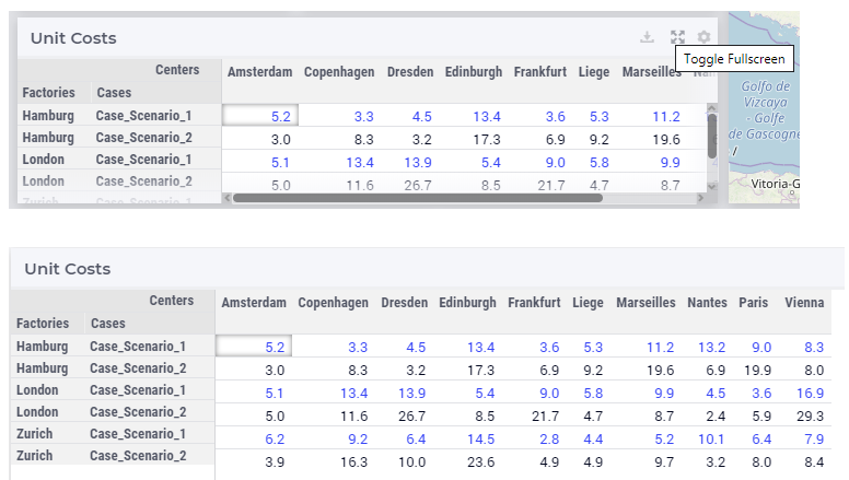
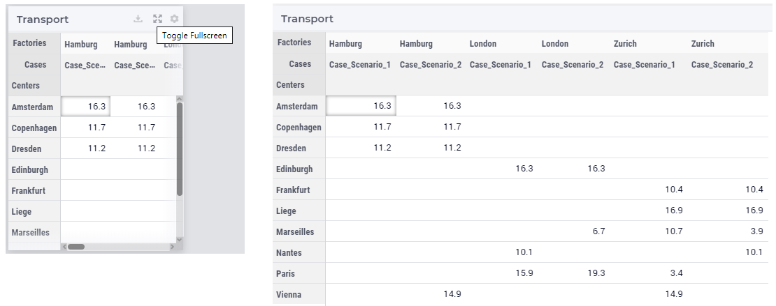
When comparing cases, some widgets show the data of both cases at the same time and therefore, the available visualization area of the widget may become insufficient for all these data to be shown without scrolling. In this case one may maximize the visualization area by using the “Toggle FullScreen” functionality of the widget, such that the data may be inspected more easily:
Now let’s keep the Case_Scenario_1 as active, but remove the case comparison with Case_Scenario_2:
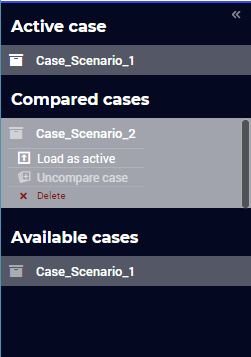
By this we move back to the situation with the initial input data and the optimization model solved.
Using widget actions and page actions
The same actions performed above using buttons may also be executed using the WebUI functionalities for widget actions or page actions.
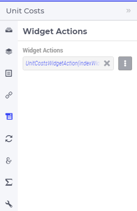
For example, for the UnitCostsData widget the action for modifying unit costs may be configured by specifying an appropriate string parameter UnitCostsWidgetAction in the Widget Actions section of the widget Settings:
This configuration string parameter should be declared and filled with some data as illustrated in this model snapshot:
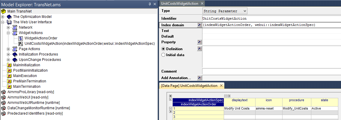
For details about declaring and filling the configuration string for the widget actions please see the Widget Actions section.
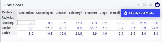
In our case at hand the specification of the widget actions introduced above results in the functionality shown below, which executes the same action as the button for modifying input data:
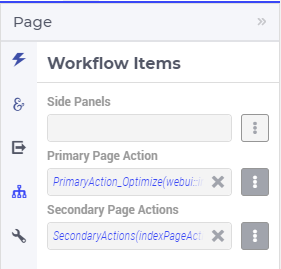
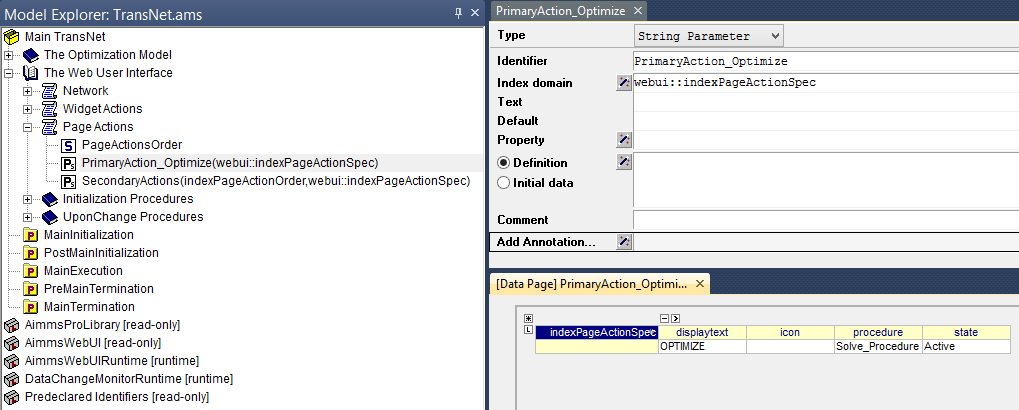
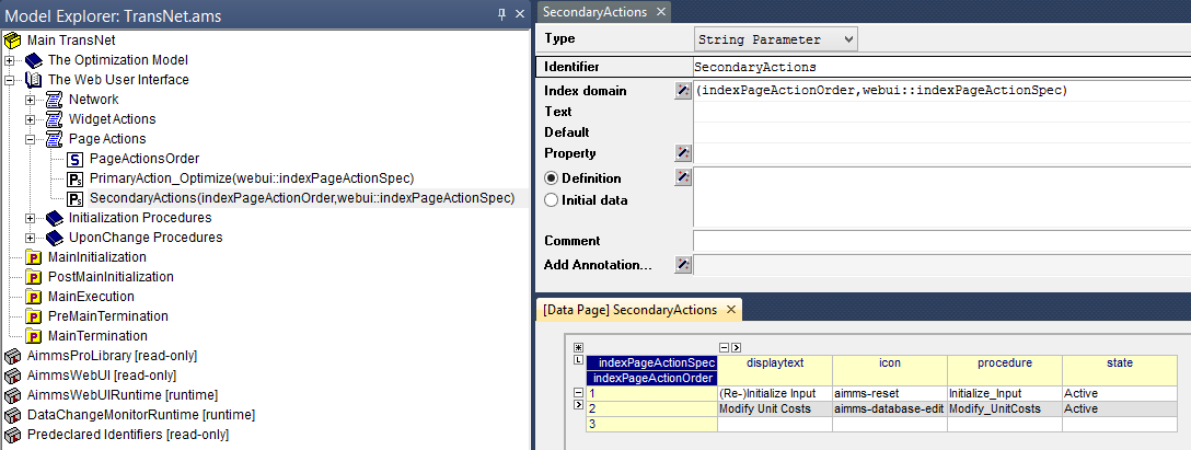
Moreover, one may specify some appropriate string parameters PrimaryAction_Optimize and SecondaryActions in the Workflow Items section of the page Settings:
The configuration string parameter for the primary page action should be declared and filled with some data as illustrated in this model snapshot:
The configuration string parameter for the secondary page actions should be declared and filled with some data as illustrated in this model snapshot:
For details about declaring and filling the configuration string for the page actions please see the Page Actions section.
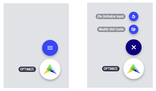
In our case at hand the specification of the page actions introduced above results in the functionality shown below, which is displayed in the bottom-right area of the application WebUI and executes the same actions as the three buttons added initially to the page:
Note
Please note that after adding widget actions or page actions executing the same procedures as some buttons on the page, the corresponding buttons may as well be removed from the page in order to free up space, possibly for other widgets to be added to the page. However, in this introductory section we chose to still keep the buttons (which became redundant) on the page purely for the sake of illustrating various WebUI functionalities.
Modifying widget types
Now one may want to visualize the input and the output data in a more graphical way. Some widgets allow to change type and show the data differently without defining a new widget for that. For example, in the Settings window of the table widgets for Supply or Demand, in the Change Type section the type may be changed, e.g., to “bar chart”, while for Transport to, e.g., “pie chart”, as shown below:
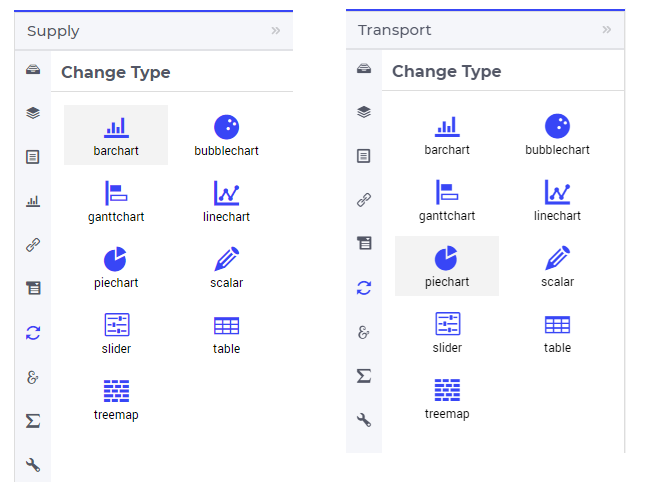
These changes lead to a WebUI as the one illustrated in the very beginning of this documentation section.
Moreover, in the created WebUI various other visualizations of the same data are possible as well. For example, if the type of the table for UnitCosts is changed to tree-map and the indexes are swapped in the order (c,f), then the final WebUI may look like in this picture:
Conclusion and final remarks
Hopefully this quick tour will give the reader a good understanding of how to start using the AIMMS WebUI. The next sections of this manual provide all the details required for building full-scope, professionally looking Web-based User Interfaces for the AIMMS applications.