Functional overview

This section

In this section you will find a description of the functionality available in the mathematical program inspector. Successively, you will learn

• the basics of the trees and windows available in the mathematical program inspector,

• how you can manipulate the contents of the variable and constraint trees through variable and constraint properties, but also using the Identifier Selector tool,

• how to inspect the contents and properties of the matrix and solution corresponding to your mathematical program, and

• which analysis you can perform using the mathematical program inspector when your mathematical program is infeasible.

Tree View Basics

Viewing generated variables and constraints

The math program inspector window displays the set of all generated variables and all generated constraints, each in a separate tree (see the left portion of Fig. 48).

In these trees, the symbolic identifiers are the first-level nodes and on every subsequent level in the tree, one or more indices are fixed. As a result, the individual variables and constraints in your model appear as leaf nodes in the two tree view windows.

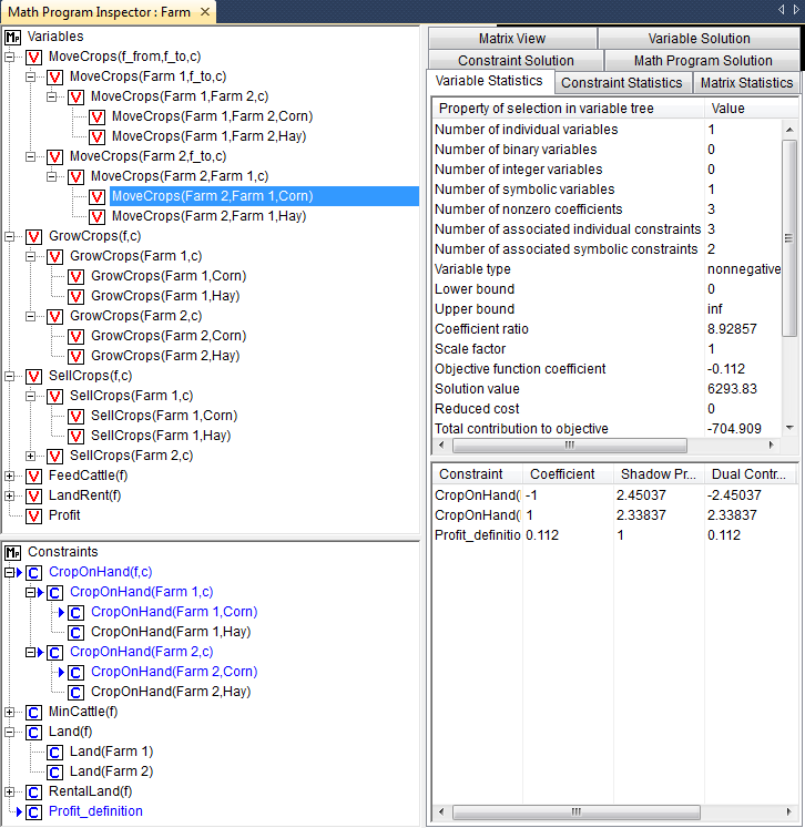
Fig. 48 The math program inspector window

Tree view selections

The math program inspector contains several tabs (see the right portion of Fig. 48) that retrieve information regarding the selection that has been made in the tree views. Common Windows controls are available to select a subset of variables and constraints (mouse click possibly in combination with the or key). Whenever you select a slice (i.e. an intermediate node in the tree) all variables or constraints in that subtree are selected implicitly. You can use the Next Leaf Node and Previous Leaf Node buttons in the toolbar for navigational purposes. In Fig. 48 a single variable has been selected in the variable tree. In addition, the text on most tabs can by copied to the Windows clipboard using the familiar Ctrl-C shortcut key.

Bookmarks

Bookmarks allow you to temporarily tag one or more variables or constraints. While navigating through the tree you will always change the current selection, while the bookmarked nodes will not be affected. Whenever you bookmark a node, all its child nodes plus parent nodes are also bookmarked. Using the Bookmarks menu you can easily select all bookmarked nodes or bookmark all selected nodes. Bookmarks appear in blue text. Fig. 48 contains a constraint tree with three bookmarked constraints plus their three parent nodes. You can use the Next Bookmark and Previous Bookmark buttons in the toolbar for navigational purposes. In case your Fig. 48 is not displayed in color, the light-gray print indicates the bookmarked selection.

Domain index display order

By default only one index is fixed at every level of the tree views, and the indices are fixed from the left to the right. However, you can override the default index order as well as the subtree depth by using the Variable Property or Constraint Property dialog on the first-level nodes in the tree. The subtree depth is determined by the number of distinct index groups that you have specified in the dialog.

Finding associated variables/ constraints

The linkage between variables and constraints in your model is determined through the individual matrix coefficients. To find all variables that play a role in a particular constraint selection, you can use the Associated Variables command to bookmark the corresponding variables. Similarly, the Associated Constraints command can be used to find all constraints that play a role in a particular variable selection. In Fig. 48, the associated constraint selection for the selected variable has been bookmarked in the constraint tree.

Advanced Tree Manipulation

Variable and constraint properties

Using the right-mouse popup menu you can access the Variable Properties and Constraint Properties. On the dialog box you can specify

• the domain index display order (already discussed above), and

• the role of the selected symbolic variable or constraint during infeasibility and unboundedness analysis.

Variable and constraint statistics

The math program inspector tool has two tabs to retrieve statistics on the current variable and constraint selection. In case the selection consists of a single variable or constraint, all coefficients in the corresponding column or row are also listed. You can easily access the variable and constraint statistics tabs by double-clicking in the variable or constraint tree. Fig. 48 shows the variable statistics for the selected variable.

Popup menu commands

In addition to Variable Properties and Constraint Properties, you can use the right-mouse popup menu to

• open the attribute form containing the declaration of an identifier,

• open a data page displaying the data of the selected slice,

• make a variable or constraint at the first level of the tree inactive (i.e. to exclude the variable or constraint from the generated matrix during a re-solve), and

• bookmark or remove the bookmark of nodes in the selected slice.

Interaction with identifier selector

Using the identifier selector you can make sophisticated selections in the variable and/or constraint tree. Several new selector types have been introduced to help you investigate your mathematical program. These new selector types are as follows.

element-dependency selector

The element-dependency selector allows you to select all individual variables or constraints for which one of the indices has been fixed to a certain element.

scale selector

The scale selector allows you to find individual rows or columns in the generated matrix that may be badly scaled. The selection coefficient for a row or column introduced for this purpose has been defined as

\[\frac{\text{largest absolute (nonzero) coefficient}} {\text{smallest absolute (nonzero) coefficient}}.\]

The Properties dialog associated with the scale selector offers you several possibilities to control the determination of the above selection coefficient.

status selector

Using the status selector you can quickly select all variables or constraints that are either basic, feasible or at bound.

value selector

The value selector allows you to select all variables or constraints for which the value (or marginal value) satisfies some simple numerical condition.

type selector

With the type selector you can easily filter on variable type (e.g. continuous, binary, nonnegative) or constraint type (e.g. less-than- or-equal, equal, greater-than-or-equal). In addition, you can use the type selector to filter on nonlinear constraints.

Inspecting Matrix Information

Variable Statistics tab

Most of the statistics that are displayed on the Variable Statistics tab are self-explanatory. Only two cases need additional explanation. In case a single symbolic (first-level node) has been selected, the Index domain density statistic will display the number of actually generated variables or constraints as a percentage of the full domain (i.e. the domain without any domain condition applied). In case a single variable (a leaf node) has been selected, the statistics will be extended with some specific information about the variable such as bound values and solution values.

Column coefficients

In case a single variable \(x_j\) has been selected, the lower part of the information retrieved through the Variable Statistics tab will contain a list with all coefficients \(a_{ij}\) of the corresponding rows \(i\), together with the appropriate shadow prices \(y_i\) (see Fig. 48). The last column of this table will contain the dual contributions \(a_{ij} y_j\) that in case of a linear model together with the objective function coefficient \(c_j\) make up the reduced cost \(\bar{c}_j\) according to the following formula.

\[\bar{c}_j = c_j - \sum_i a_{ij} y_i\]

Nonlinear coefficients

Coefficients of variables that appear in nonlinear terms in your model are denoted between square brackets. These numbers represent the linearized coefficients for the current solution values.

Constraint Statistics tab

The Constraints Statistics tab and the Variable Statistics tab retrieve similar statistics. Fig. 49 shows the constraint statistic for the selection consisting of a single constraint. Note that in this particular case the symbolic form of the constraint definition will also be displayed. In case the selected constraint is nonlinear, the individual nonlinear constraint as generated by AIMMS and communicated to the solver is also displayed.

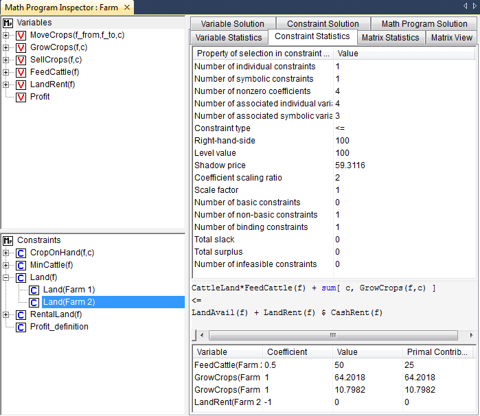
Fig. 49 The math program inspector window

Row coefficients

In case a single row \(i\) has been selected, the lower part of the Constraint Statistics tab will contain all coefficients \(a_{ij}\) in the corresponding columns \(j\), together with their level values \(x_j\). The last column of this table lists the primal contributions \(a_{ij} x_j\) that together in case of a linear model with the right-hand-side make up either the slack or surplus that is associated with the constraint according to the following formula.

\[\mathrm{slack}_i - \mathrm{surplus}_i = \mathrm{rhs}_i - \sum_j a_{ij} x_j\]

Nonlinear constraints

As is the case on the Variable Statistics Tab, all coefficients corresponding to nonlinear terms are denoted between square brackets. For these coefficients, the last column displays all terms that contribute to the linearized coefficient value.

Matrix Statistics tab

The Matrix Statistics tabs retrieves information that reflects both the selection in the variable tree and the selection in the constraint tree. Among these statistics are several statistical moments that might help you to locate data outliers (in terms of size) in a particular part of the matrix.

Matrix View tab

The Matrix View tab contains a graphical representation of the generated matrix. This view is available in two modes that are accessible through the right-mouse popup menu. The symbolic block view displays at most one block for every combination of symbolic variables and symbolic constraints. The individual block view allows you to zoom in on the symbolic view and displays a block for every nonzero coefficient in the matrix. It is interesting to note that the order in which the symbolic and individual variables and constraints are displayed in the block view follows the order in which they appear in the trees.

Block coloring

The colors of the displayed blocks correspond to the value of the coefficient. The colors will vary between green and red indicating small and large values. Any number with absolute value equal to one will be colored green. Any number for which the absolute value of the logarithm of the absolute value exceeds the logarithm of some threshold value will be colored red. By default, the threshold is set to 1000, meaning that all nonzeros \(x \in (- \infty,-1000] \;\cup\; [- \frac{1}{1000},\frac{1}{1000}] \;\cup\; [1000,\infty)\) will be colored red. All numbers in between will be colored with a gradient color in the spectrum between green and red.

Block patterns

Any block that contains at least one nonlinear term will show a hatch pattern showing diagonal lines that run from the upper left to the lower right of the block.

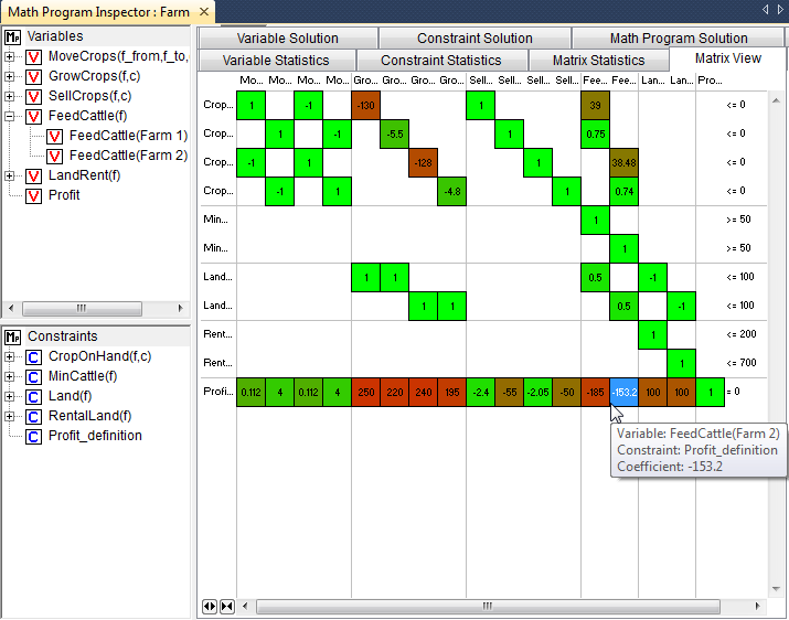
Fig. 50 The matrix view (individual mode)

AIMMS option

The value of the threshold mentioned in the previous paragraph is available as an AIMMS option with name bad_scaling_threshold and can be found in the Project - Math program inspector category in the AIMMS Options dialog box.

Block tooltips

While holding the mouse inside a block, a tooltip will appear displaying the corresponding variables and constraints. In the symbolic view the tooltip will also contain the number of nonzeros that appear in the selected block. In the individual view the actual value of the corresponding coefficient is displayed.

Block view features

Having selected a block in the block view you can use the right-mouse popup menu to synchronize the trees with the selected block. As a result, the current bookmarks will be erased and the corresponding selection in the trees will be bookmarked. Double-clicking on a block in symbolic mode will zoom in and display the selected block in individual mode. Double-clicking on a block in individual mode will center the display around the mouse.

Block coefficient editing

When viewing the matrix in individual mode, linear coefficient values can be changed by pressing the F2 key, or single clicking on the block containing the coefficient to be changed.

Inspecting Solution Information

Solution tabs

The tabs discussed so far are available as long as the math program has been generated. As soon as a solution is available, the next three tabs reveal more details about this solution.

Variable Solution tab

The Variable Solution tab shows the following seven columns

• Variable Name,

• Lower Bound,

• Value (i.e. solution/level value),

• Upper Bound,

• Marginal (i.e. reduced cost),

• Basis (i.e. Basic, Nonbasic or Superbasic), and

• Bound (i.e. At bound or In between bounds).

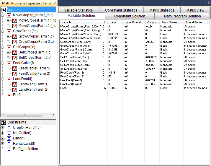
Fig. 51 The variable solution

By clicking in the header of a column you can sort the table according to that specific column.

Constraint Solution tab

A similar view is available for the constraints in your mathematical program. The Constraint Solution tab contains the following five columns

• Constraint Name,

• Value (i.e. solution),

• Marginal (i.e. shadow price),

• Basis (i.e. Basic, Nonbasic or Superbasic), and

• Bound (i.e. Binding or Nonbinding).

Solution related AIMMS options

By default AIMMS will only store marginal solution values if explicitly specified in the Property attribute (through the ReducedCost or ShadowPrice property). An more convenient way to ensure that all marginal solution information is available to the math program inspector is by setting the option Store_complete_solver_solution_tree to yes. When the nonlinear presolver has been activated (by setting the Nonlinear_presolve option (in the Solvers General category) to on), the option Store_nonlinear_presolve_info has to be set yes to make sure that the math program inspector is able to display information about the reductions that have been achieved by the nonlinear presolver.

Math Program Solution tab

The Math Program Solution tab retrieves solution information about the mathematical program that has been solved. This information is similar to that in the AIMMS Progress window.

Logging messages

The lower part of the information retrieved by this tab is used to display logging messages resulting from the Bound Analysis and Unreferenced Identifiers commands in the Actions menu.

Solving MIP models

Whenever your linear model is a mixed-integer model, the solver will most probably use a tree search algorithm to solve your problem. During the tree search the algorithm will encounter one or more solutions if the model is integer feasible. Once the search is completed, the optimal solution has been found.

MIP Search Tree tab

With the MIP Search Tree tab you can retrieve branching information about the search tree. Only CPLEX and GUROBI provide this information. In addition the option Show_branch_and_bound_tree has to be set to on (before the solve) to instruct AIMMS to store search tree information during the solve.

Improving the search process

The size and shape of the search tree might give you some indication that you could improve the performance of the solver by tuning one or more solver options. Consider the case in which the search tree algorithm spends a considerable amount of time in parts of the tree that do not seem interesting in retrospect. You might consider to use priorities or another branching rule, in an attempt to direct the search algorithm to a different part of the tree in an earlier stage of the algorithm.

Controlling search tree memory usage

Because all structural and statistical information is kept in memory, displaying the MIP search tree for large MIPs might not be a good idea. Therefore, you are able to control to the and size of the stored search tree through the option Maximum_number_of_nodes_in_tree.

Search tree display

For every node several solution statistics are available. They are the sequence number, the branch type, the branching variable, the value of the LP relaxation, and the value of the incumbent solution when the node was evaluated. To help you locate the integer solutions in the tree, integer nodes and their parent nodes are displayed in blue.

Incumbent progress

The lower part of the MIP Search Tree tab retrieves all incumbent solutions that have been found during the search algorithm. From this view you are able to conclude for example how much time the algorithm spend before finding the optimal solution, and how much time it took to proof optimality.

Performing Analysis to Find Causes of Problems

Unreferenced identifiers

One of the causes of a faulty model may be that you forgot to include one or more variables or constraints in the specification of your mathematical model. The math program inspector helps you in identifying some typical omissions. By choosing the Unreferenced Identifiers command (from the Actions menu) AIMMS helps you to identify

• constraints that are not included in the constraint set of your math program while they contain a reference to one of the variables in the variable set,

• variables that are not included in the variable set of your math program while a reference to these variables does exist in some of the constraints, and

• defined variables that are not included in the constraint set of your math program.

The results of this action are visible through the Math program solution tab.

A priori bound analysis

In some situations it is possible to determine that a math program is infeasible or that some of the constraints are redundant even before the math program is solved. The bound analysis below supports such investigation.

Implied constraint bounds

For each linear constraint with a left-hand side of the form

\[\sum_j a_{ij} x_j\]

the minimum level value \(\underline{b_i}\) and maximum level value \(\overline{b_i}\) can be computed by using the bounds on the variables as follows.

\[\begin{split}\begin{aligned} \underline{b_i} & = & \sum_{j|a_{ij}>0} a_{ij} \underline{x_j} + \sum_{j|a_{ij}<0} a_{ij} \overline{x_j} \\ \overline{b_i} & = & \sum_{j|a_{ij}>0} a_{ij} \overline{x_j} + \sum_{j|a_{ij}<0} a_{ij} \underline{x_j}\end{aligned}\end{split}\]

Performing bound analysis

By choosing the Bound Analysis command (from the Actions menu) the above implied bounds are used not only to detect infeasibilities and redundancies, but also to tighten actual right-hand-sides of the constraints. The results of this analysis can be inspected through the Math Program Solution tab. This same command is also used to perform the variable bound analysis described below.

Implied variable bounds \(\ldots\)

Once one or more constraints can be tightened, it is worthwhile to check whether the variable bounds can be improved. An efficient approach to compute implied variable bounds has been proposed by Gondzio [Gon94], and is presented without derivation in the next two paragraphs.

\(\ldots\) for \(\leq\) constraints

For \(i\) in the set of constraints of the form \(\sum_j a_{ij} x_j \leq b_i\), the variable bounds can be tightened as follows.

\[\begin{split}x_k & \leq \underline{x_k} + \min_{ i | a_{ik} > 0} \frac{b_i - \underline{b_i}}{a_{ik}} \\ x_k & \geq \overline{x_k} + \max_{ i | a_{ik} < 0} \frac{b_i - \underline{b_i}}{a_{ik}}\end{split}\]

\(\ldots\) and \(\geq\) constraints

For \(i\) in the set of constraints of the form \(\sum_j a_{ij} x_j \geq b_i\), the variable bounds can be tightened as follows.

\[\begin{split}x_k & \leq \underline{x_k} + \min_{ i | a_{ik} < 0} \frac{b_i - \overline{b_i}}{a_{ik}} \\ x_k & \geq \overline{x_k} + \max_{ i | a_{ik} > 0} \frac{b_i - \overline{b_i}}{a_{ik}}\end{split}\]

Phase 1 analysis

In case infeasibility cannot be determined a priori (e.g. using the bound analysis described above), the solver will conclude infeasibility during the solution process and return a phase 1 solution. Inspecting the phase 1 solution might indicate some causes of the infeasibility.

Currently infeasible constraints

The collection of currently infeasible constraints are determined by evaluating all constraints in the model using the solution that has been returned by the solver. The currently infeasible constraints will be bookmarked in the constraint tree after choosing the Infeasible Constraints command from the Actions menu.

Substructure causing infeasibility

To find that part of the model that is responsible for the infeasibility, the use of slack variables is proposed. By default, the math program inspector will add slacks to all variable and constraint bounds with the exception of

• variables that have a definition,

• zero variable bounds, and

• bounds on binary variables.

Adapting the use of slack variables

The last two exceptions in the above list usually refer to bounds that cannot be relaxed with a meaningful interpretation. However these two exceptions can be overruled at the symbolic level through the Analysis Configuration tab of the Properties dialog. These properties can be specified for each node at the first level in the tree. Of course, by not allowing slack variables on all variable and constraint bounds in the model, it is still possible that the infeasibility will not be resolved.

Slack on variable bounds

Note that to add slacks to variable bounds, the original simple bounds are removed and (ranged) constraints are added to the problem definition.

\[\underline{x_j} \leq x_j + s^+_j - s^-_j \leq \overline{x_j}\]

Elastic model

After adding slack variables as described above, this adapted version of the model is referred to as the elastic model.

Minimizing feasibility violations

When looking for the substructure that causes infeasibility, the sum of all slack variables is minimized. All variables and constraints that have positive slack in the optimal solution of this elastic model, form the substructure causing the infeasibility. This substructure will be bookmarked in the variable and constraint tree.

Irreducible Inconsistent System (IIS)

Another possibility to investigate infeasibility is to focus on a so-called irreducible inconsistent system (IIS). An IIS is a subset of all constraints and variable bounds that contains an infeasibility. As soon as at least one of the constraints or variable bounds in the IIS is removed, that particular infeasibility is resolved.

Finding an IIS

Several algorithms exist to find an irreducible inconsistent system (IIS) in an infeasible math program. The algorithm that is used by the AIMMS math program inspector, if the option Use_IIS_from_solver is disabled, is discussed in Chinneck ([Chi91]). Note that since this algorithm only applies to linear models, the menu action to find an IIS is not available for nonlinear models. While executing the algorithm, the math program inspector

1. solves an elastic model,

2. initializes the IIS to all variables and constraints, and then

3. applies a combination of sensitivity and deletion filters.

Deletion filtering

Deletion filtering loops over all constraints and checks for every constraint whether removing this constraint also solves the infeasibility. If so, the constraint contributes to the infeasibility and is part of the IIS. Otherwise, the constraint is not part of the IIS. The deletion filtering algorithm is quite expensive, because it requires a model to be solved for every constraint in the model.

Sensitivity filtering

The sensitivity filter provides a way to quickly eliminate several constraints and variables from the IIS by a simple scan of the solution of the elastic model. Any nonbasic constraint or variable with zero shadow price or reduced cost can be eliminated since they do not contribute to the objective, i.e. the infeasibility. However, the leftover set of variables and constraint is not guaranteed to be an IIS and deletion filtering is still required.

Combined filtering

The filter implemented in the math program inspector combines the deletion and sensitivity filter in the following way. During the application of a deletion filter, a sensitivity filter is applied in the case the model with one constraint removed is infeasible. By using the sensitivity filter, the number of iterations in the deletion filter is reduced.

Substructure causing unboundedness

When the underlying math program is not infeasible but unbounded instead, the math program inspector follows a straightforward procedure. First, all infinite variable bounds are replaced by a big constant \(M\). Then the resulting model is solved, and all variables that are equal to this big \(M\) are bookmarked as being the substructure causing unboundedness. In addition, all variables that have an extremely large value (compared to the expected order of magnitude) are also bookmarked. Any constraint that contains at least two of the bookmarked variables will also be bookmarked.

Options

When trying to determine the cause of an infeasibility or unboundedness, you can tune the underlying algorithms through the following options.

• In case infeasibility is encountered in the presolve phase of the algorithm, you are advised to turn off the presolver. When the presolver is disabled, solution information for the phase 1 model is passed to the math program inspector.

• During determination of the substructure causing unboundedness or infeasibility and during determination of an IIS, the original problem is pertubated. After the substructure or IIS has been found, AIMMS will restore the original problem. By default, however, the solution that is displayed is the solution of the (last) pertubated problem. Using the option Restore_original_solution_after_analysis you can force a resolve after the analysis has been carried out.

• Solvers like CPLEX and GUROBI have their own algorithm to calculate an IIS. If the option Use_IIS_from_solver is switched on, its default setting, then AIMMS will retrieve an IIS calculated by the solver. If this option is switched off then AIMMS will use its own algorithm based on Chinneck ([Chi91]), as described above.

Scaling

A coefficient matrix is considered badly scaled if its nonzero coefficients are of different magnitudes. Scaling is an operation in which the variables and constraints in the model are multiplied by positive numbers resulting in a matrix containing nonzero coefficients of similar magnitude. Scaling is used prior to solving a model for several reasons, the most important being (1) to improve the numerical behavior of the solver and (2) to reduce the number of iterations required to solve the model.

Scale model

Solvers like CPLEX and GUROBI use their own algorithms to scale a model but in some cases it might be beneficial to use a different scaling algorithm that uses symbolic information. The scaling tool in the math program inspector can be used to find scaling factors for all symbolic variables and constraints in the model by selecting the Scale Model command from the Actions menu. The scaling factors will be displayed in the Scaling Factors tab. Once the scaling tool is finished you can select the Resolve command from the Actions menu to resolve the model which then automatically uses these scaling factors. However, to use the scaling factors in your AIMMS model you have to manually update the Unit attribute of the corresponding variables and constraints.